ERT Data
Some main functionalities related the ERT Data projects can be found in the window that opens automatically when the program is launched. Clicking with the right mouse button on the Home node and then on the action tool, the window can be opened again (Figure 82).
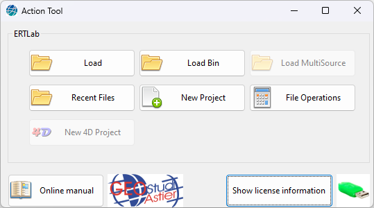
Figure 82 Action Tool panel
According to the type of license activated (see the green USB protection dongle) the number of buttons shown and activated can change.
At the bottom of that window it can be found a small image that tells if the USB dongle is insert (the image is coloured) or not (the image is greyed). If it is needed to check if the USB dongle status it can be pressed the button Show license information, if there is any problem the message shown should be similar to Figure 83.
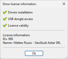
Figure 83 Show license information
At the bottom of that window there is also a button to open the Online manual, in case of needs.
The main buttons available in the tool window are:
Load: opens a *.DATA file, a project that has already been created and saved.
Recent Files: opens a recently opened project.
Load Bin: loads a *.BIN file, a field data file collected with IRIS Syscal instruments. See the Conversion table for a smarter file import.
Load Multisource: this is an additional package to process datasets acquired using the multi-source methodology (measurements are made while multiple dipoles transmit simultaneously). It loads a *.wDat file, a field data file collected with MTP-IRIS Multisource instruments.
New Project: opens an empty project, it adds the Data node to the tree but without loading any data files.
File Operation: loads two projects and makes operations between them; it is a useful tool for time lapse evaluation (to compare the resistivity response before and after an event).
New 4D Project: this is an additional package to run time-lapse inversions using the differences approach.
File Operation
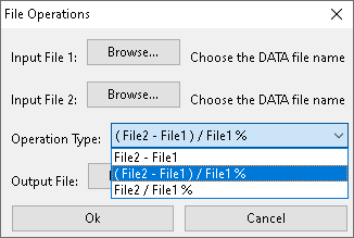
Figure 84 File Operation
It is needed to specify the input DATA file name 1 and 2, where it will be loaded the 3D models (usually obtained from an inversion, see section Inversion ).
It is also needed to specify the type of operation that needs to be used to combine the input meshes. Usually this tool is used to compute a percentage variation, so the option shown in the Figure 84 it is then used.
An output file is then saved (in the location specified), and then it is automatically opened to view the results immediately.
It is quite common to set the colormap shown in Figure 85 , being also careful to put identical extremes so that the zero value is associated with the white colour.
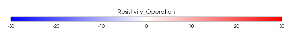
Figure 85 Colormap example
Timelapse 4D Project
Warning
Feature not available in the basic license; included in the “4D” add-on.
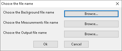
Figure 86 New 4D Project
To create a 4D project it is needed to specify two input DATA filenames. These derive from the saving of measurements that took place at different times. The purpose of this tool is to help achieve a stable joint inversion, to evaluate the differences in the model. The requirement is to use electrodes in exactly the same position, and the sequence of measurements must be identical (or as similar as possible). The first file is defined “Background”, it is usually temporally prior to the other, that is defined “Measurements”.
The “Background” DATA file name must contain:
Electrodes and field measurements
A Model, obtained from the 3D inversion of the field data
The inversion parameters used to get the Inverted
The calculated data obtained from the forward model computed on the Model and the measurement sequence given
Note that all these information are always available automatically after an usual processing from the field data to the inverted model.
The “Measurements” DATA file name must contain:
The same electrodes and field sequence measurement.
Any mesh and inverted model needs to be provided in the “Measurements” DATA, also any other parameter need to be specified (for example parameters to compute the mesh, or to perform the inversion).
As usual, raw data cannot be used to successfully complete an inversion process, but a filter operation must be performed. Since this step will most likely bring, for each measurement, a different number of surviving quadrupoles, then the program will autonomously identify the subset common to the two files in order to correctly set the 4D project. In order to carry out any analysis on this step, a copy of “Background” and “Measurements” DATA file it is then saved, storing only the common quadrupoles, it is added the postfix “_Updated” to the original name.
The output 4D project is then saved in the location specified, then it is automatically opened by ERTLab Studio. It is then only needed to run the inversion process, without editing the parameters given (taken automatically from the “Background” DATA project). At the end, the inverted 3D model will be available for viewing, which can also be compared with the reference model (“Background”) by percentage variation (see section File Operation ).
Obviously, a similar result can also be obtained by comparing separate classic inversions of the two available data, but since the two inversions will be independent in this way, then it is known that many more artifacts will appear from the comparison of the results. The 4D method helps to have more homogeneous inversions, and to considerably mitigate the presence of such artifacts.
Main project node
An ERT project will create in the tree the node ERT data. Whatever kind of file is opened, a lot of nodes are added to the tree, as child of ERT data.
In Figure 87 the new node created in the tree, and its property panel.
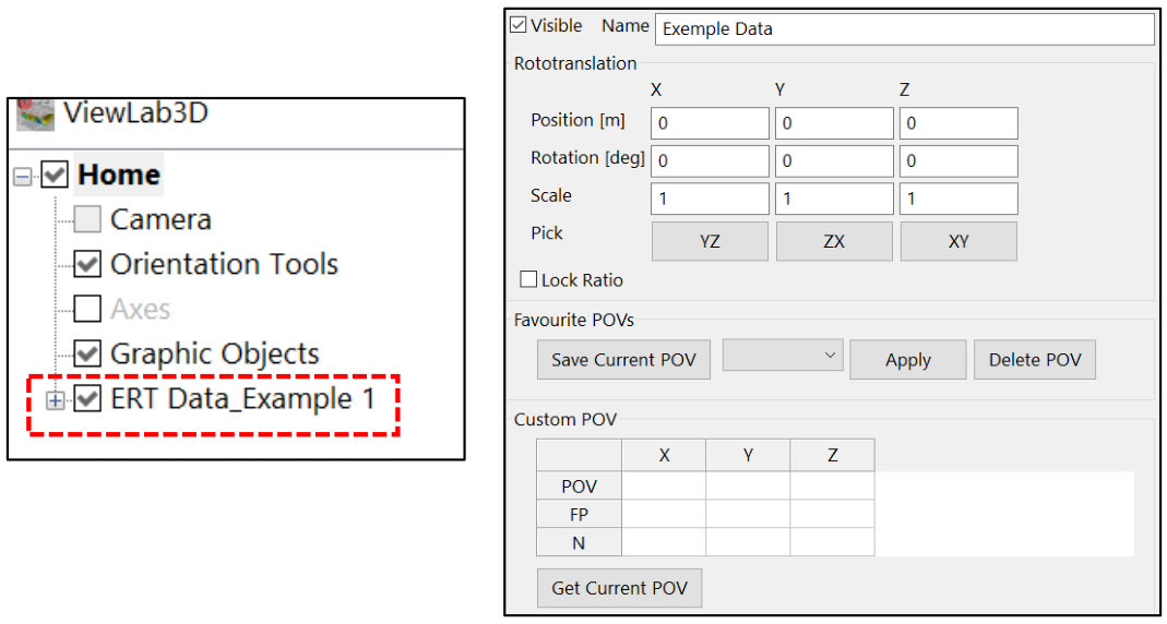
Figure 87 ERT Data panel
Note that the Name of the project was renamed to ERT data_Example 1. It can be also set if the project needs to be Visible or not. With Centre Camera to this the user can automatically place the selected project at the centre of the scene. It is particularly useful in those cases when many projects are loaded and the selected one is not visible, because it is out the scene (by default, the scene is centred to view all the objects in the scene).
A Rototranslation can be set to the entire project. This is only a “graphic” rototranslation, the actual coordinates of the data file do not change. It is a useful tool to visualize the project in a coordinates reference system different from the one the data were collected in. For example, in the case that the axes are in a new coordinate system, but you can still export the data file, nothing has changed and it is still in the original coordinate system or to make some quick evaluation tests to find the correct rototranslation values to apply to the ERT data to actually rototranslate it through the proper tool (see Rototranslation).
As it is available in the node Camera, it is possible to manage some Favourite POVs. Note that the Favourite POVs will be stored automatically when the ERT project will be saved, else the Favourite POVs in the Camera node will be lost when the program is closed.
Clicking with the right mouse button in the ERT Data node it is possible to:
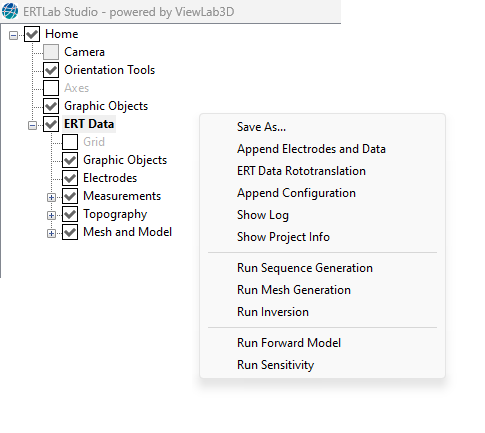
Figure 88 ERT Data tools
Save As: through this button it is possible to save the Data-File at any time.
Append Electrodes and Data: through this tool the user can append electrodes and data belonging to another data file to the current project. It is useful to merge two or more ERT lines together.
Merging two or more lines into one project can be accomplished in two different way:
It is possible to load the first file with Load/Load Bin/Load Multisource and then add the second file through the “Append Electrodes and Data” tool. In this way the project maintains the name of the first loaded project (but it is possible to change it in the Name box later)
It is also possible to create an empty project with the New Project button and then upload all the file together through the “Append Electrodes and Data” tool. In this way the project maintains the default name ERT Data (but it is possible to change it in the Name box later)
Append Configuration: through this option the user can append the configuration used in another previous project to the current project. This includes all the setting of the Run Mesh Generation and the Run Inversion Panels.
ERT Data Rototranslation: this tool enacts an effective rototranslation of the dataset. It is unlike the graphic rototranslation and in above in this paragraph (ERT Data panel) (see Rototranslation). Using this tool and then exporting data loses the original reference system at the favor of a new coordinate system.
Show Project Info: it opens a window with the File Summary (Figure 89). Information about the number of electrodes and measurements of the project, the dimension of the mesh and the possible presence of topography file, and Resistivity/IP/Sensitivity Models are reported. Originally, Resistivity IP and Sensitivity are “Empty” because no inversion has been computed yet. When a Resistivity/IP inversion is computed the proper menu items become enabled, because it is recognized the presence of an inverted Model. For the IP menu there is an intermediate state: “Homogeneous”. It suggests that there is a unique IP value coming from the generation of the mesh (and therefore the project contains IP measurements), but the inversion has not been computed yet. In the following table all the possible cases are summarized.
Empty |
Homogeneous |
Found |
|
RESISTIVITY |
There is no inverted Resistivity model in the project |
__ |
The project contains a Resistivity model which came from an inversion process |
IP |
There is no inverted IP model in the project |
The project contains an homogeneous IP value, but there is no inverted IP model yet |
The project contains an IP model which came from an inversion process |
SENSITIVITY |
There is no calculated Sensitivity model in the project |
__ |
The project contains a calculated Sensitivity model |
In the example in Figure 89 the loaded project:
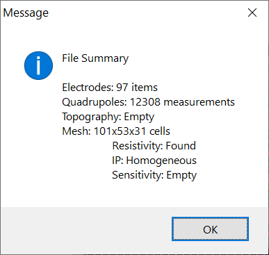
Figure 89 Example of Summary File message
contains 97 Electrodes;
contains 12308 Measurements;
has no topography information (Topography: Empty);
the Mesh has been calculated (accordingly the IP menu it is “Homogeneous”) and it is composed by 101 x 53 x 31 cells;
contains a Resistivity Model, which came from an inversion already computed (Resistivity: Found);
doesn’t contain an IP Model, but a homogeneous IP value is present, which came from the mesh generation;
doesn’t contain a calculated Sensitivity Model (Sensitivity: Empty).
Other commands available in the ERT Data node are:
Run Sequence Generation: see Run Sequence Generation.
Run Mesh Generation: see Run Mesh Generation.
Run Inversion: see Run Inversion.
Run Forward Model: see Run Forward Model.
Run Sensitivity: see Run Sensitivity.
This main node “ERT Data” represents the entire project and is composed of other menu items, which are described in more detail below.
Grid
This node has exactly the same functionalities of the Grid node available into the Graphic Objects node.
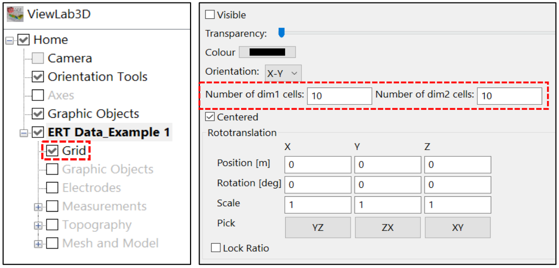
Figure 90 Grid Panel in ERT Data node
Graphic Object
This element is completely analogous to that described Graphic Objects , refer to it for more information.
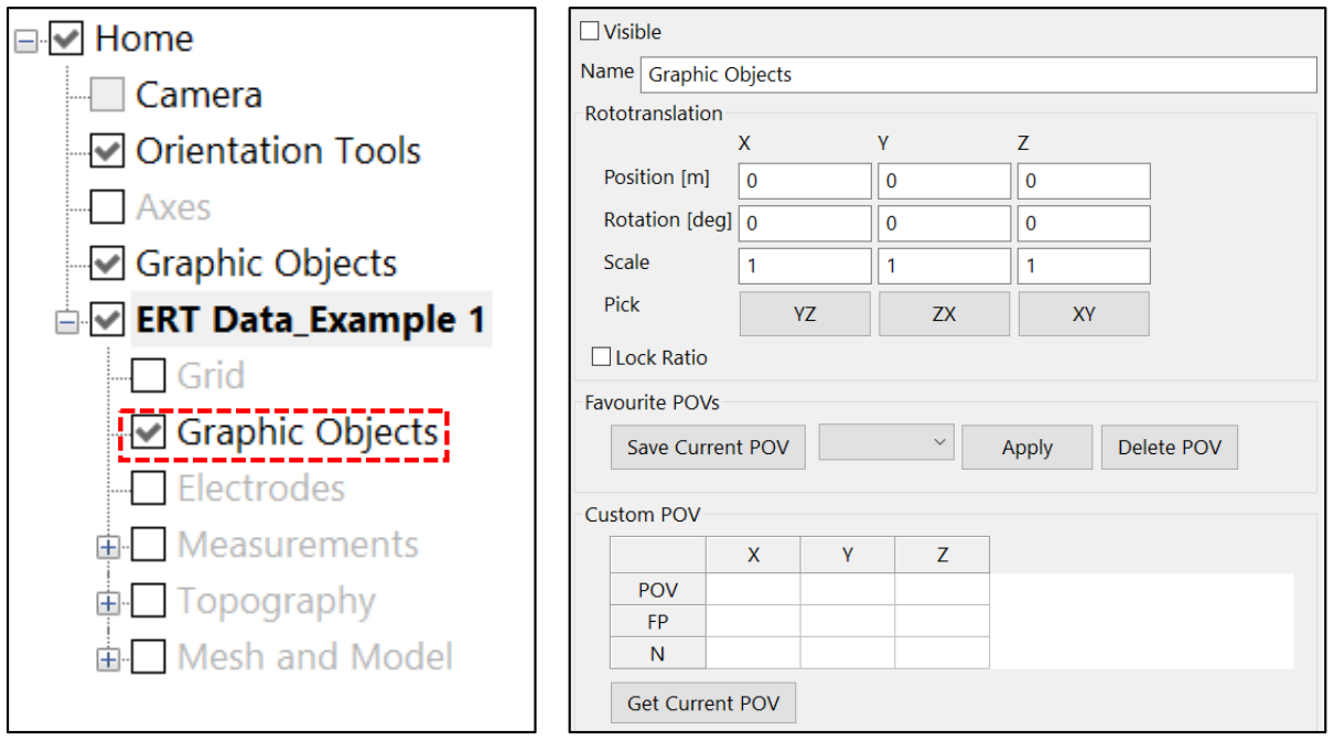
Figure 91 Graphic object panel
The graphic objects added in this menu belongs to the project. Each graphical modification applied to it involved the objects too. For example, if the project is rototranslate, the objects are rototranslate too. Otherwise, if objects are added in the node as explained in Graphic Objects, they are unlinked from the project, so they do not move.