Mesh and Model
This menu option has the purpose of modelling the subsurface with a 3D grid (mesh) and to assign physical properties values(model) to the points of this half-space.
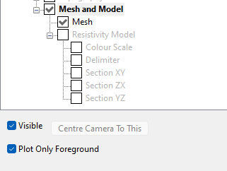
Figure 114 Mesh and Model properties
If “Plot Only Foreground” is checked the Background region is not visible; otherwise the entire mesh is visualized.
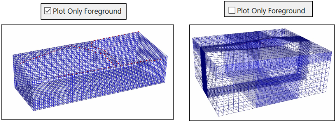
Figure 115 On the left, mesh with “Plot Only Foreground” flagged; on the right, mesh with “Plot Only Foreground” not flagged, so also the background region is displayed.
There can be some child nodes, which are explained below.
Mesh
This option manages the way of the mesh representation. The window has the following items:
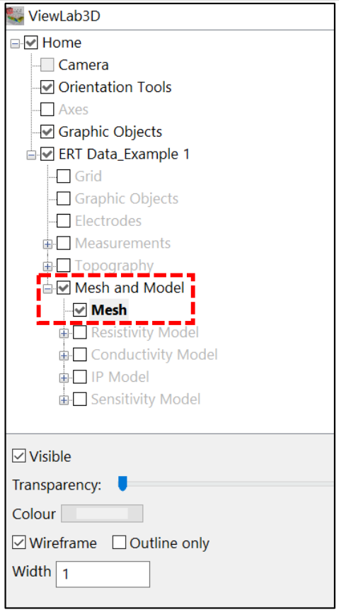
Figure 116 Mesh panel
Visible
The checkbox controls the visibility of the mesh.
Transparency
Through the slider the transparency of the mesh, as it is shown can be controlled (Figure 117).
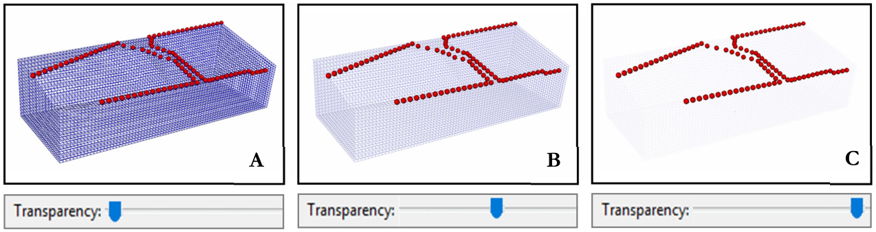
Figure 117 Example of different levels of transparency of the mesh
Colour
By default the mesh is grey, but it can be changed to any colour. Figure 118 shows a change from grey to green.
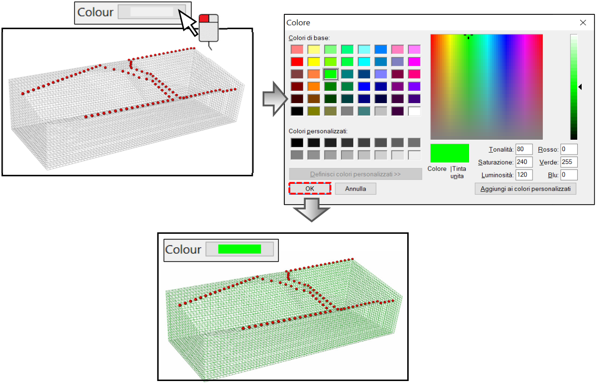
Figure 118 Example of mesh colour change
Wireframe
If the Wireframe box is checked the mesh is visible as lines. If Outline only is checked too, the mesh is visualized with just the external lines (case A in Figure 119). If Outline only is not checked the mesh is visualized with every cell that constitutes the entire volume (case B in Figure 119). If both the boxes are unchecked the volume is visualized as a “solid” body (case C in Figure 119).
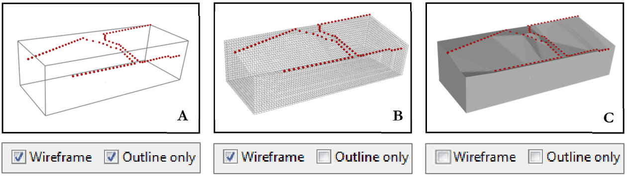
Figure 119 Example of different combination of ‘wireframe’ and ‘outline only’ mesh visualization mode
Width
If Wirefram e is selected, the width of the mesh can be chosen by typing a number from 1 to 10 or through the slider which appears clicking on the box. Two different outline widths are shown in Figure 120.
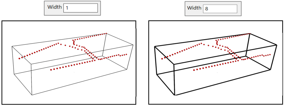
Figure 120 Example of different mesh widths
Resistivity Model
The Resistivity Model quantifies how strongly the investigated body contrasts the flow of electric current. The Resistivity Model is present in the project after the inversion process has been run (Figure 121).
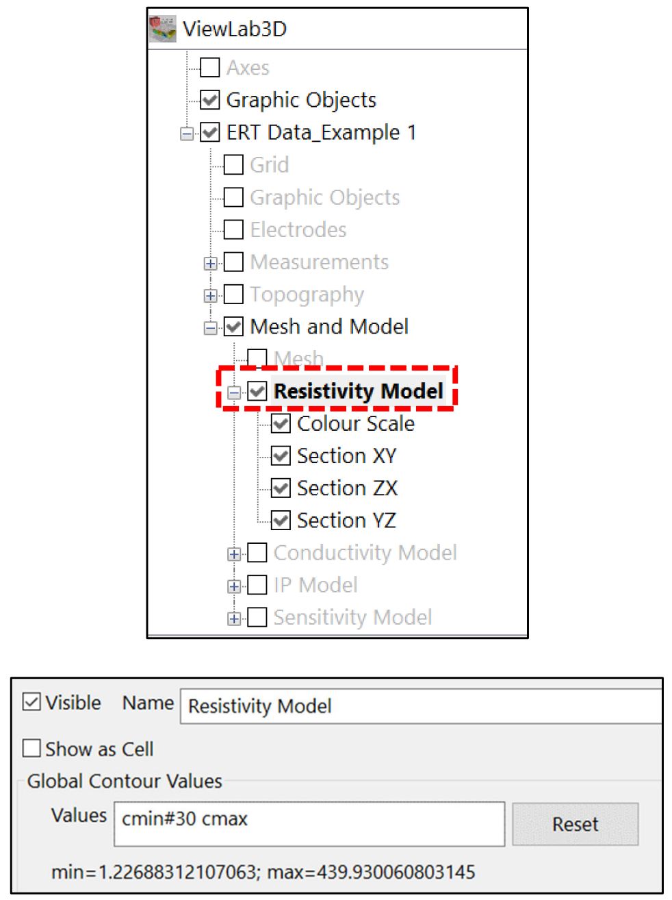
Figure 121 Resistivity Model panel
Visible
This checkbox controls the Resistivity Model visibility;
Name
By default, the node name is labeled “Resistivity Model”, but it possible to change it by typing the desired new name in this box;
Show as cell
If this checkbox is selected, the model is shown composed by cells. Otherwise it is represented as an interpolation of points. The model obtained in this last case is smoother (Figure 122).
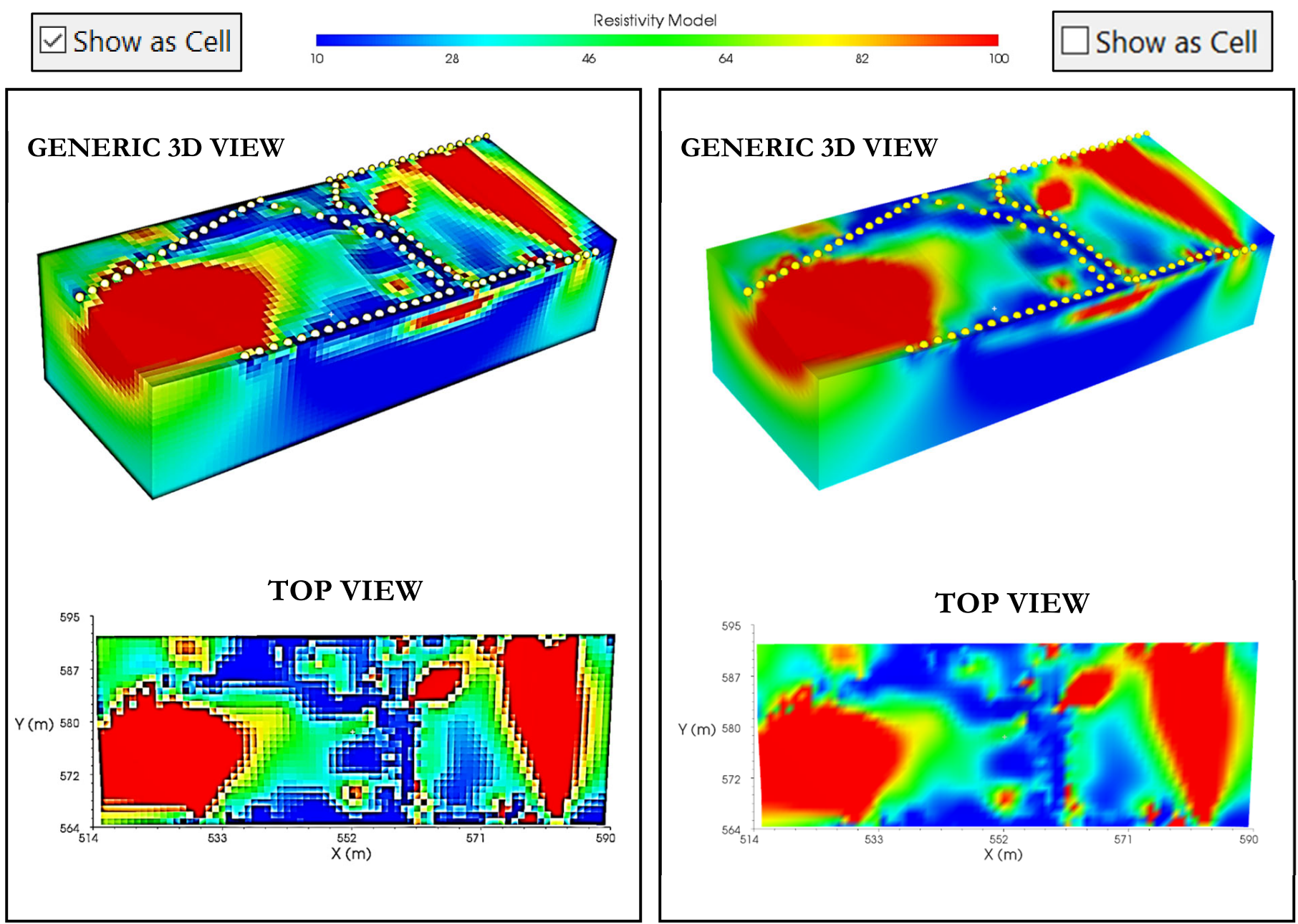
Figure 122 Examples of Resistivity Model with “show as cells” checked on the left and not checked on the right
Global Contour Values
Manages the contour lines of all sections inserted in the Resistivity Model. The maximum and minimum value to apply at the contouring and the step interval within one line and the other can be selected. In the lower part of the box the minimum and maximum value of the entire dataset is automatically reported.
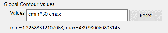
Figure 123 Resistivity Model sub-panel
These values are applied to each section, but it is possible to change them and set custom values to each section, as is shown in this section.
Sub nodes
Colour Scale: allows to set the properties of the colour scale as described in the Colour Scale section.
Delimiter: allows to show only a portion of the available mesh, see the Delimiter section.
Section XY-ZX-YZ: there are three predefined sections, one for each main direction XY, XZ, YZ.
Clicking with the right mouse button on the Resistivity Model node it is possible to add some additional nodes. They are:
Sections: see Model Section
Volume: see Model Volume
Isosurface: see Model Isosurface
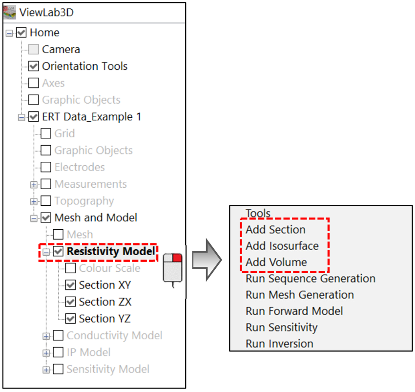
Figure 124 Add Section/Isosurface/Volume to the Resistivity Model
Examples
To close out this section we visualize more Resistivity Model examples in Figure 125 and Figure 126 to show some of the many data representation possibilities.
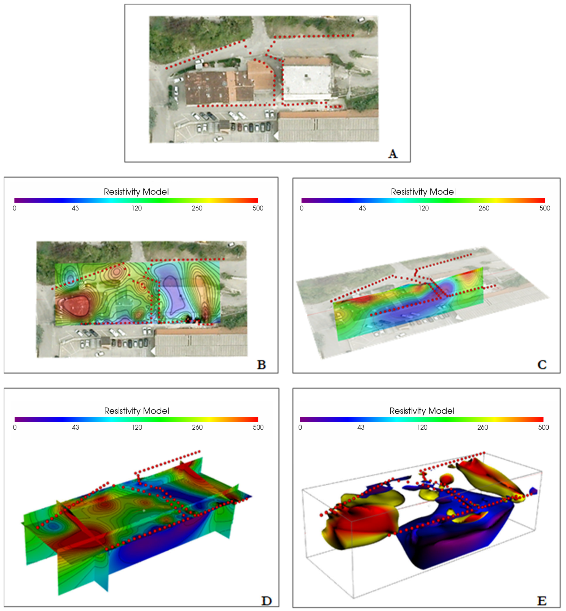
Figure 125 Some of many resistivity model project visualization possibilities. In A, aerial photo of the investigated site (from Google Earth) overlaid to electrodes used for the acquisition; in B visualization of Resistivity Model through the insertion of a XY section; in C insertion of a YZ section; in D insertion of 5 sections, 2 parallel to the YZ plane, 2 to XZ plane and 1 to XY plane; in E visualization of the mesh (outline only) and two volumes, one incorporating the most conductive areas (5-15 ohm*m, in blue) and the other the most resistive area (80-150 ohm*m, in yellow-red)
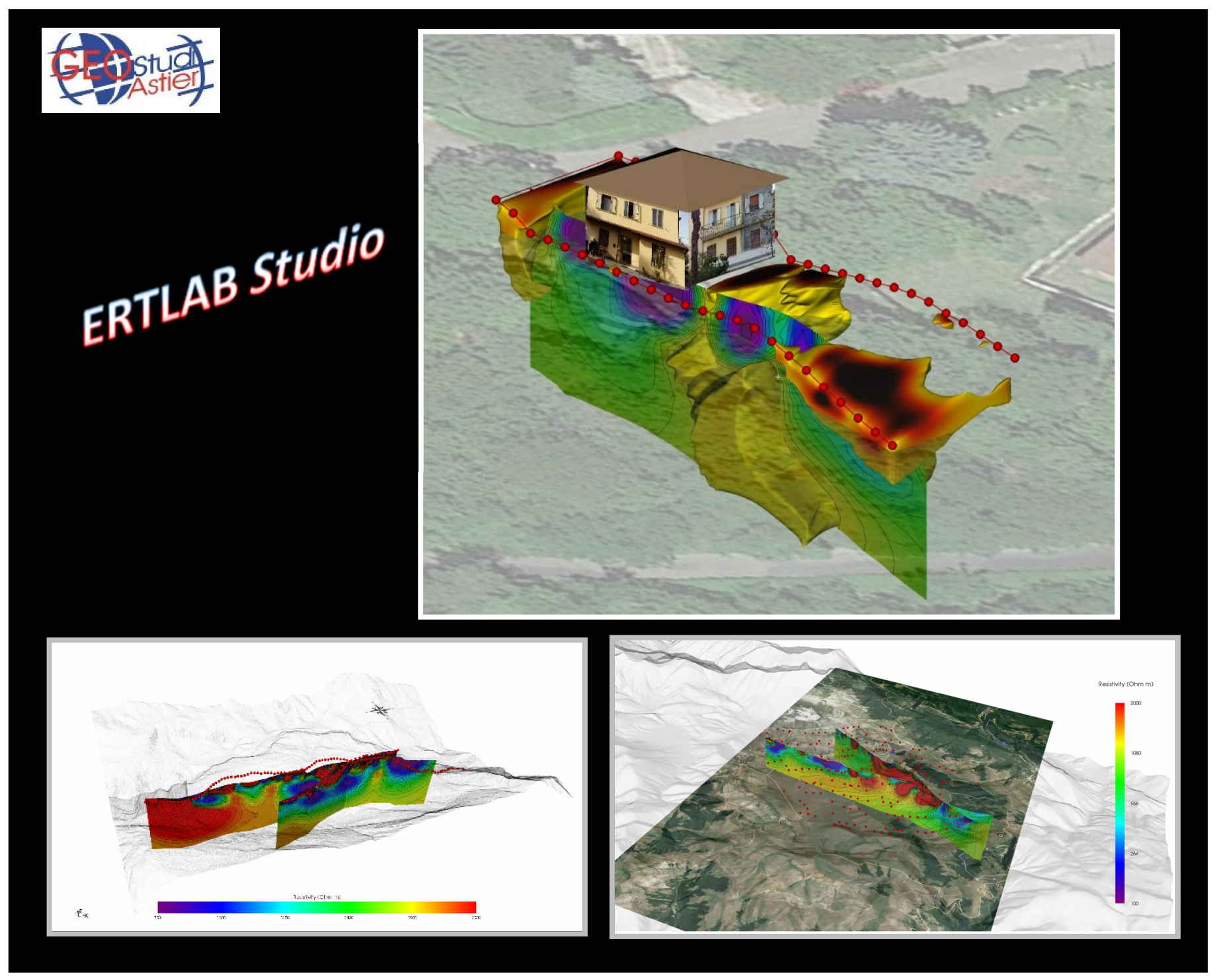
Figure 126 At the top, example of resistivity sections with aerial photo , electrodes, resistivity volume and custom building; on the bottom left, example of resistivity sections with electrodes and topography. On the bottom right example of resistivity section with electrodes, topography and aerial photo.
Conductivity Model
The Conductivity Model quantifies how easily the material allows the flow of electric current. It is the reciprocal of the resistivity model. As illustrated in Figure 127 the areas that are showing the maximum values in the conductivity model show minimum values in the conductivity model and vice versa.
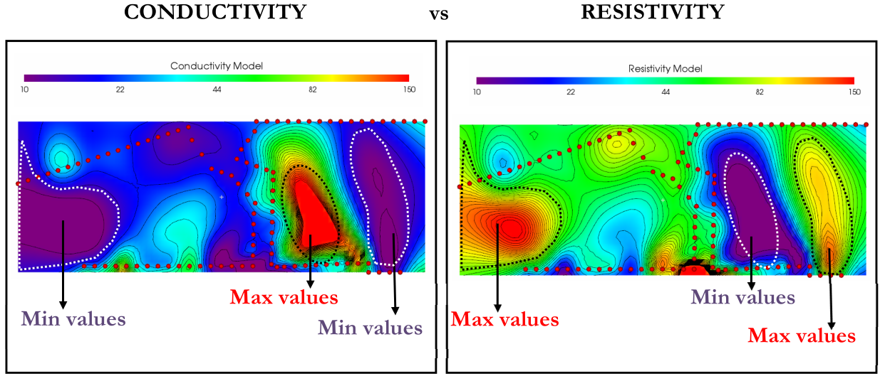
Figure 127 Comparison between Conductivity and Resistivity Models.
All its options are the same as those of the Resistivity Model section.
IP Model
In the IP methodology the ground is energized with an alternating square wave pulse and it consists in measuring the IP effect as a time-diminishing voltage at the receiver electrodes. The method is based on the observation of potential curve decay subsequent to the interruption of the input current, that is the extent of the “residual chargeability” retained by the soil under investigation. All its sub menus and options are the same of the Resistivity Model section.
Metal Factor Model
Warning
Feature not available in the basic license; included in the “Graphics pack” add-on.
This model is computed automatically based on the Resistivity and the chargeability (IP) models currently available. It is obtained dividing IP by Resistivity, and then a multiplier factor 1000 is applied to get more readable values. All its sub menus and options are the same of the Resistivity Model section.
Sensitivity Model
The sensitivity model indicates how much the variations of resistivity of subsurface will influence the potential measured by the electrode array. It provides an estimate of how much the electrical property of the ground must vary to produce significant effects on the measurement. Different arrays have different sensitivity patterns, some of them describe the superficial levels better others the deeper levels. To compute the sensitivity of the electrode configuration of the loaded project (just one quadrupoles or all quadrupoles together) use the Run Sensitivity option. In Figure 128 the area in red shows the maximum sensitivity, areas where collected data will be more reliable. The areas in purple are not optimally covered, as expected as the area with maximum sensitivity correspond to the area where the electrodes (yellow spheres in Figure 128) are positioned.
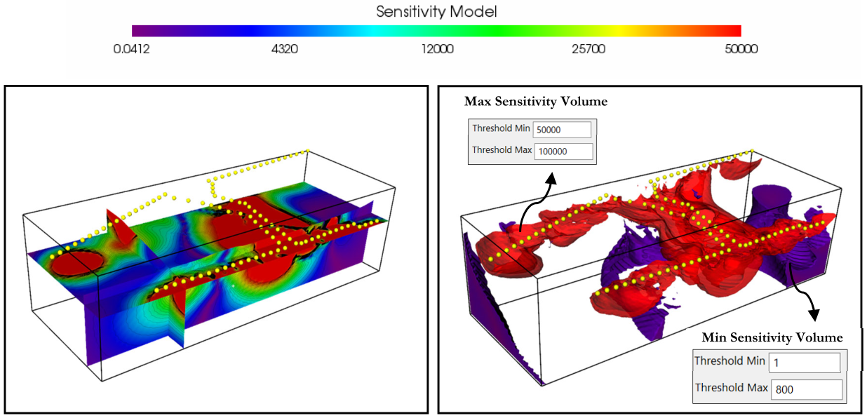
Figure 128 Sections and volumes of Sensitivity Model
Delimiter
Warning
Feature not available in the basic license; included in the “Graphics pack” add-on.
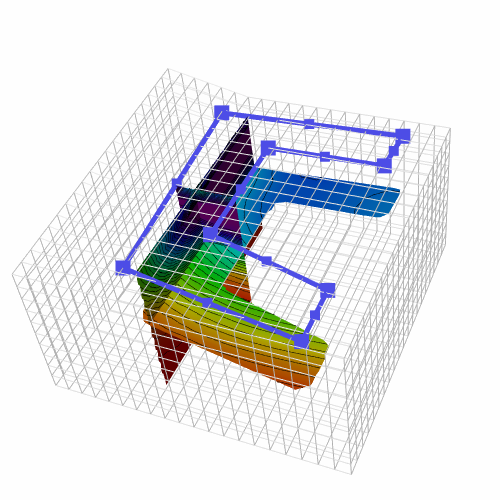
Figure 129 Delimiter
With this tool it is possible to show only the most interesting part of the mesh. To define how the mesh needs to be resized a polyline has to be defined.
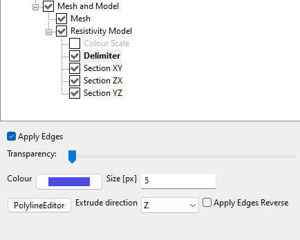
Figure 130 Delimiter parameters
It is possible to set the Transparency, Colour and the Size (in pixel) of the polyline provided. However the polyline is shown only when the Polyline Editor is open.
Apply Edges
Controls if the Delimiter is enabled, that means that it needs to effectively cut the mesh or not.
Polyline Editor
Same tool described here.
The only difference is that in this case the polyline is closed, that means that the first and last point provided are connected with an additional segment.
Extrude direction
Sets the direction (in the 3D space) where the polyline needs to be projected. The options are:
X: The polyline is extruded horizontally, along X axis.
Y: The polyline is extruded horizontally, along Y axis.
Z: The polyline is extruded vertically, along Z axis (default).
Automatic: The polyline is automatically extruded perpendicular to the mean plane on which it lies.
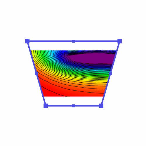
Figure 131 Delimiter example with horizontal extrusion to remove the corners to a 2D section
Apply Edge Reverse
To control which part (inner or outer) of the mesh to be shown with respect the polyline provided.
In Figure 128 is shown:
A Delimiter disabled, shown the original mesh
B Delimiter active, with Apply Edge Reverse disabled
C Delimiter active, with Apply Edge Reverse enabled
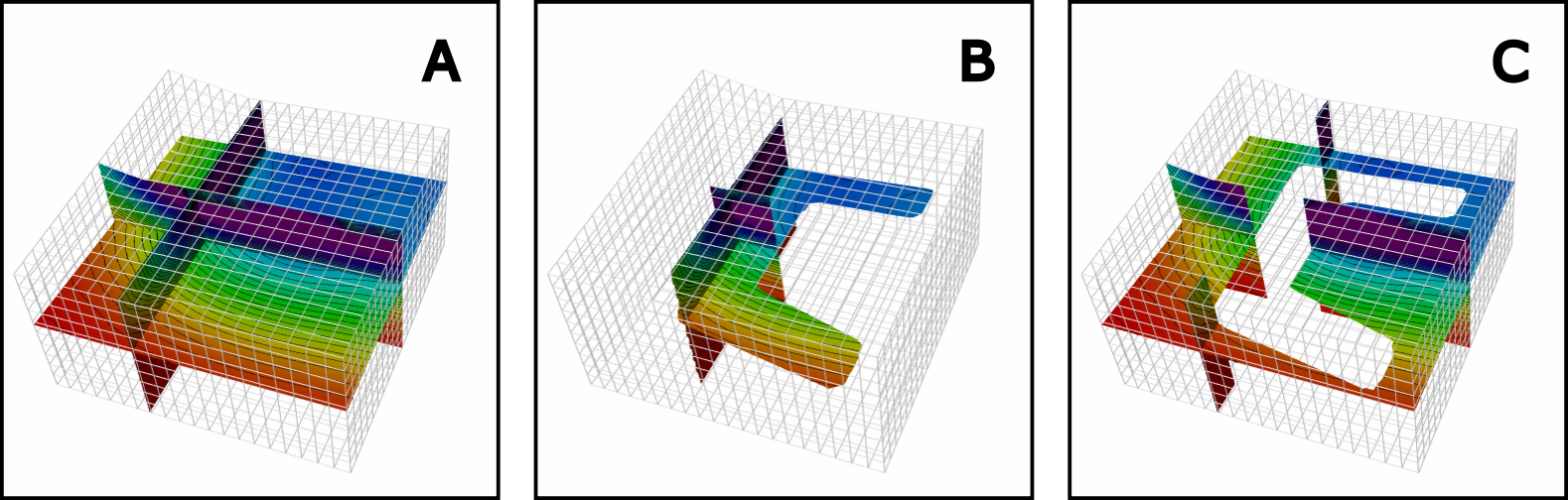
Figure 132 Delimiter examples