Run Mesh Generation

By clicking with the right mouse button on the main node of the “ERT Data”, and choosing “Run Mesh Generation” opens a new window that lets the user configure the mesh.

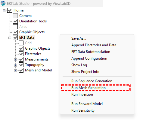
Figure 293 Run Mesh Generation

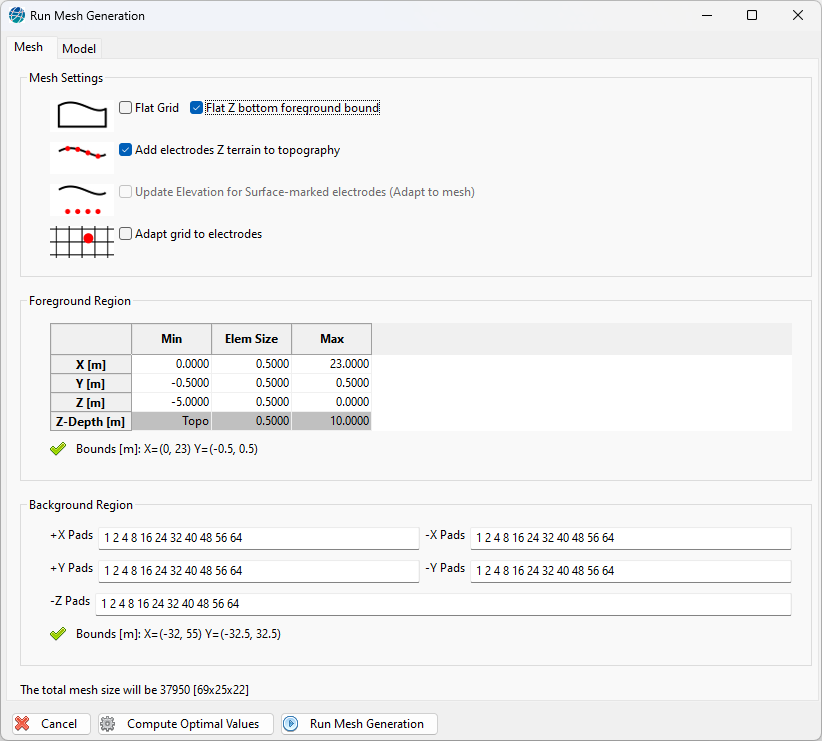
Figure 294 Mesh generation panel

The mesh generation window has two tabs: Mesh and Mode.

The Mesh tab is in turn divided into three main areas: Mesh Setting, Foreground Region and Background Region.

Mesh

Mesh Setting

In this area there are options for setting the mesh in relation to the topography and the positioning of the electrodes in the 3D space.

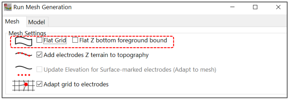
Figure 295 Shape of the mesh

If Flat Grid is active, the top and the bottom of the mesh surface are flat, so there is no topographic information. Otherwise, if the Flat Grid is inactive, the top of the mesh follows the topography. The geometry of the bottom of mesh is set by “Flat Z bottom foreground bound” option. If selected, the bottom of the mesh is flat, otherwise it also follows the topography trend. The icons of the tool changes in function depending on the users selection helping to make the right choice. In summary, there are three possible cases:

• 1° case: Flat Grid selected:

In this case, the mesh is flat so there is no topographic information.

• 2° case: Flat Grid not selected, Flat Z bottom selected:

In this case the top of the mesh follows the topography. The volume of the individual cells of the mesh do not change, so there will be parts of the mesh with cells more “stretched” and areas with cells more “squeezed”.

• 3° case: Flat Grid not selected, Flat not Z bottom selected:

In this case both the top and the bottom of the mesh follow the topography, so the thickness of the mesh is constant, and the cells have all the same size. These three cases are illustrated in Figure 296, where there is a simple synthetic case on the left and a more complex real case on the right.

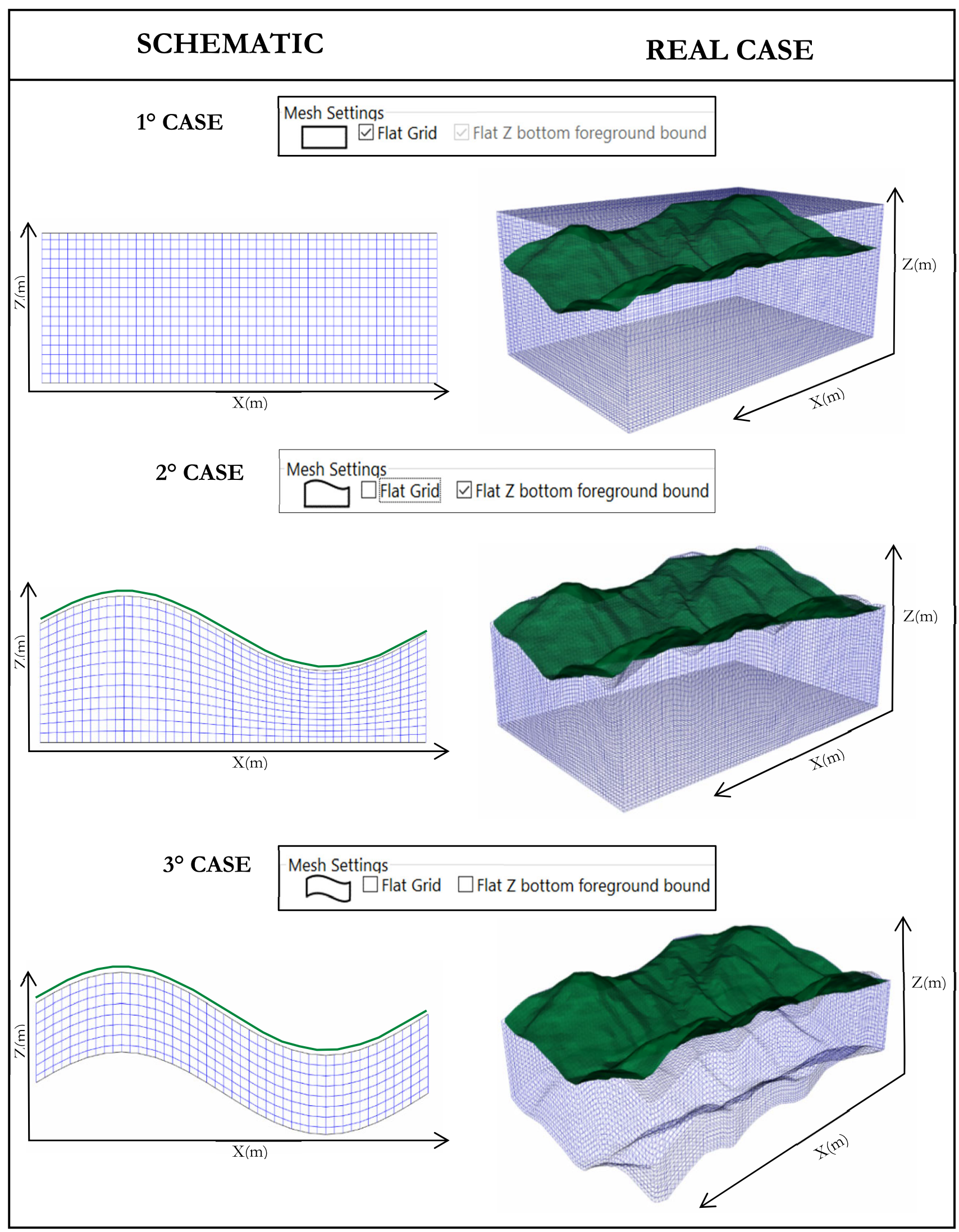
Figure 296 Examples of different kinds of mesh

If the mesh has the topographic information (previous case 2 and 3), it may happen that the z coordinates of one or more electrodes are not consistent with the topography file. In most cases, the Z information of the topography is more accurate than the Z value of the electrodes. To adapt the electrodes to the mesh you can select the appropriate check box:

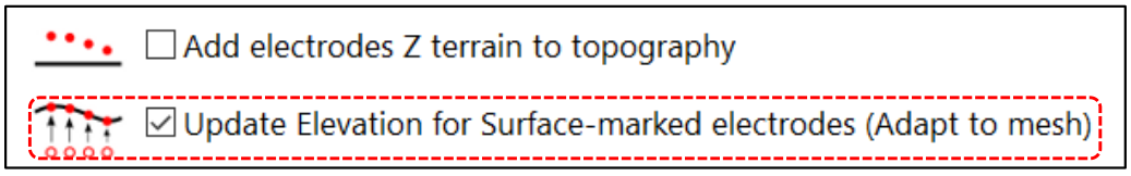
Figure 297 Adapt electrodes elevation to mesh

If for some reason the Z of the electrodes must be taken into consideration, e.g. if the topography file is not a DEM (Digital Elevation Model) and just composed of some scattered points, it is possible to add the electrode Z terrain to the topography file, through the dedicated check box:

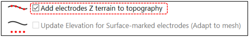
Figure 298 Add electrodes elevation to topography

Figure 299 shows a schematic example, with an unrealistic gap between the information of the Z value of the electrodes and the Z of the topography, The electrodes follow a sinusoidal shaped curve and the topography is instead flat. In the left case the “Add electrodes Z terrain to topography” is selected, so the electrodes remain fixed and the mesh changes shape to adapt to the Z electrodes trend. If “Update Elevation for Surface marked electrodes (Adapt to Mesh)” is selected, the mesh remains flat and the electrodes move to its surface (on the right in Figure 299).

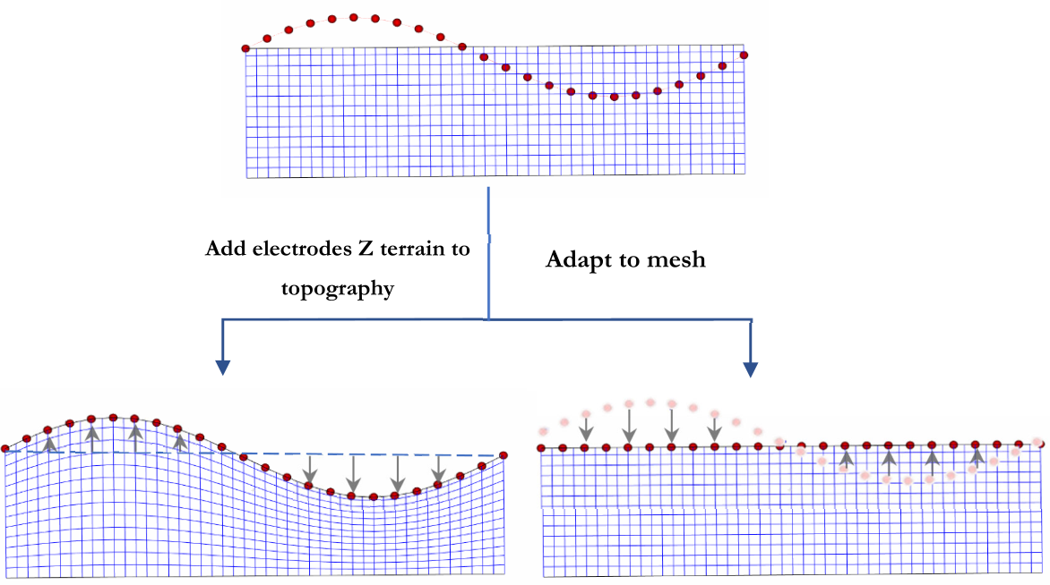
Figure 299 Examples of different kind of mesh in relation to the rule of the Z electrodes information

If there is a topography file loaded, selecting “Add electrodes Z terrain to topography” is deduced from the Z electrodes coordinates information. The last tool of the Mesh Setting tab manages the position of an electrode in relation to the node mesh position, in the XY plane.

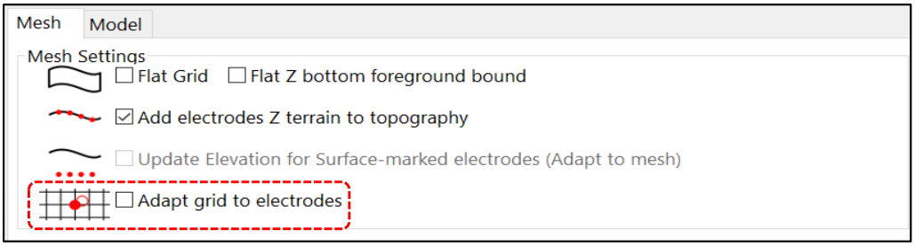
Figure 300 Adapt grid to electrodes

In fact, it is possible that the position of one or more electrodes does not coincide with any node of the mesh, as in the following example (Figure 301). In this case it is possible to distort the mesh so that the electrodes position coincide with its nodes.

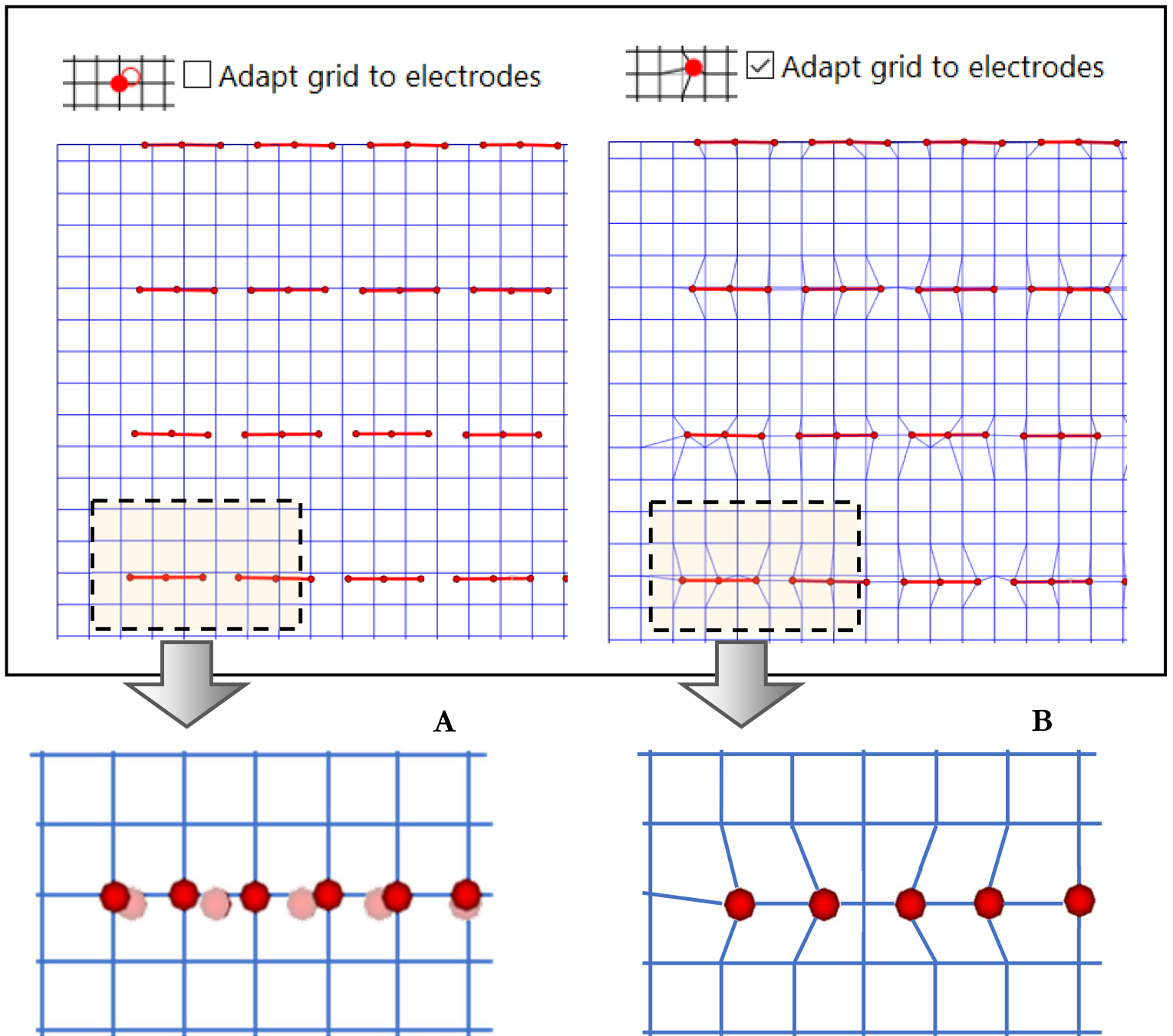
Figure 301 In A, “Adapt grid to electrode” is not checked so the electrodes not coincident with the node moves on the nearest node; in B “Adapt grid to electrode” is flagged so the mesh is deformed to adapt the node to the position of the electrodes, which does not change position

Foreground Region

The mesh is divided into two main areas, the background and the foreground region. The Foreground Region (red area in Figure 302) is the portion of the mesh which includes the investigated area and is defined by the geometry of the electrodes on the ground; outside is the Background Region which defines an area necessary for the mitigation of the boundaries effects, theoretically infinite.

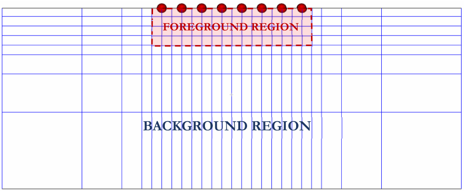
Figure 302 Background and Foreground regions

It is possible to set the values of the Foreground Region through the dedicated table show. By default, the limits values are the same as the maximum and minimum electrodes coordinates and the size of the cell is half the minimum electrodes distance of the data set. To obtain these default values click on “Compute Optimum Value” button. Doing so, the software will compute the more appropriate values for the table, basing on the electrodes spacing.

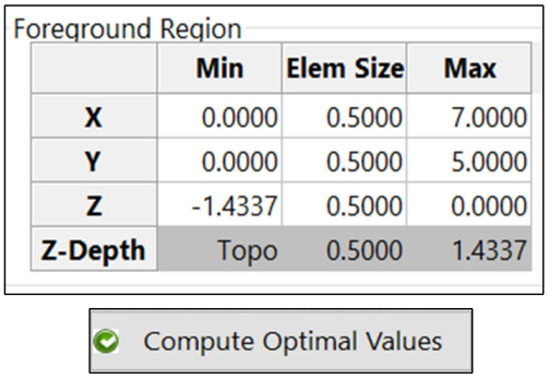
However, it is possible to change these values typing the desired numbers in the table. It is advisable to check the Element Size dimension because it may be excessively small. This can happen if for logistical reasons two electrodes were placed in the ground at a distance significantly lower than all the other electrodes, the software will consider half of this minimum distance as the size of the cells of the entire mesh. For example, if all the electrodes are at 2 m distance of each other except 2 electrodes, which are at 0.4m of distance, the correct cell size value is 1m and not 0.2 m as the software suggests (Figure 303).

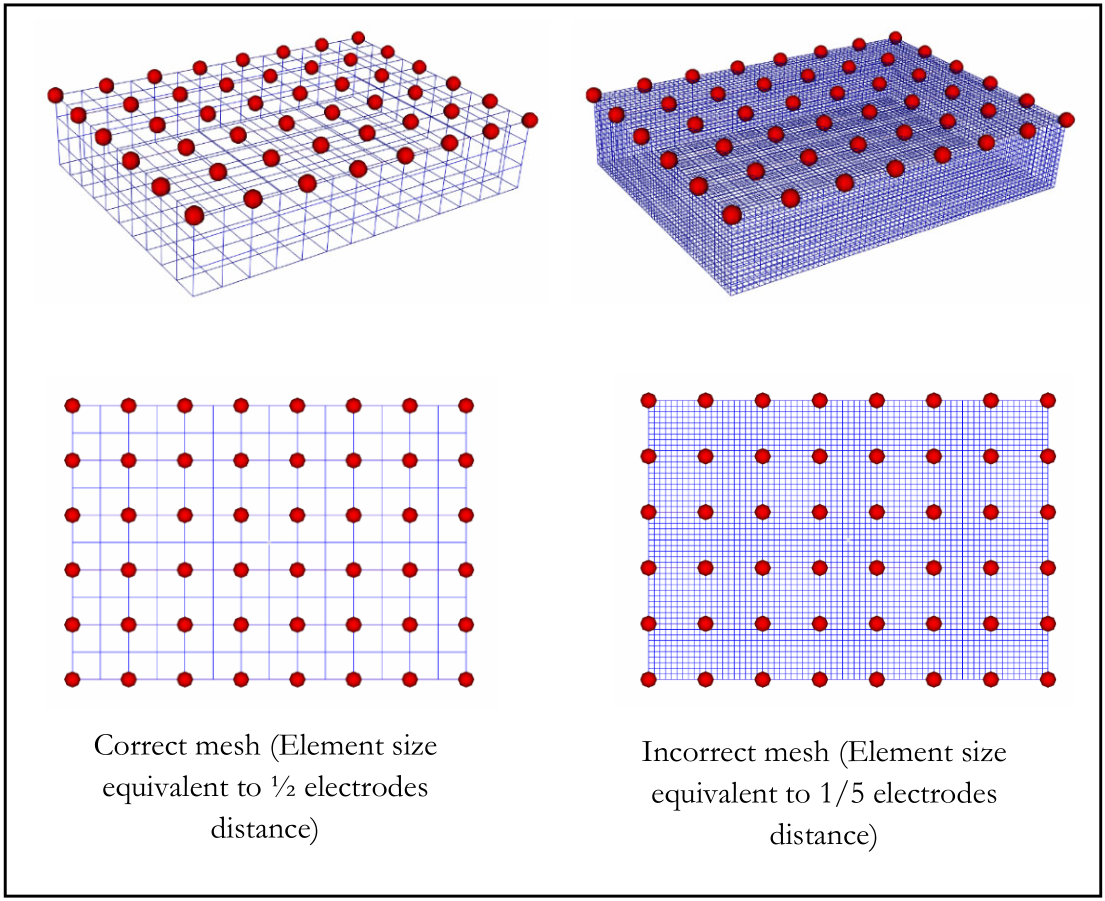
Figure 303 Example of two mesh with different cell sizes

If the bottom of the mesh is flat, the Z-Depth is not editable and the corresponding row is greyed out, because there is not a constant thickness only a minimum and maximum value of the Z (the positive values are above the surface and the negative underground). Alternatively, if the bottom of the mesh follows the topography the thickness is constant, so the Z-Depth is editable (Figure 304).

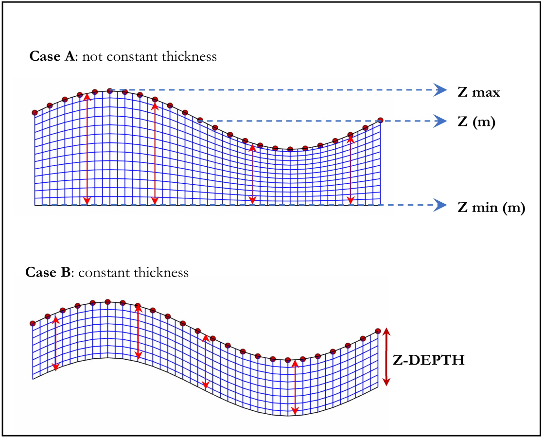
Figure 304 Mesh_Z parameter setting

In Figure 305 an example is shown of a Foreground Region generated by the values reported in the table; the distance between electrodes is 1m, so the size of the cells is 0.5m.

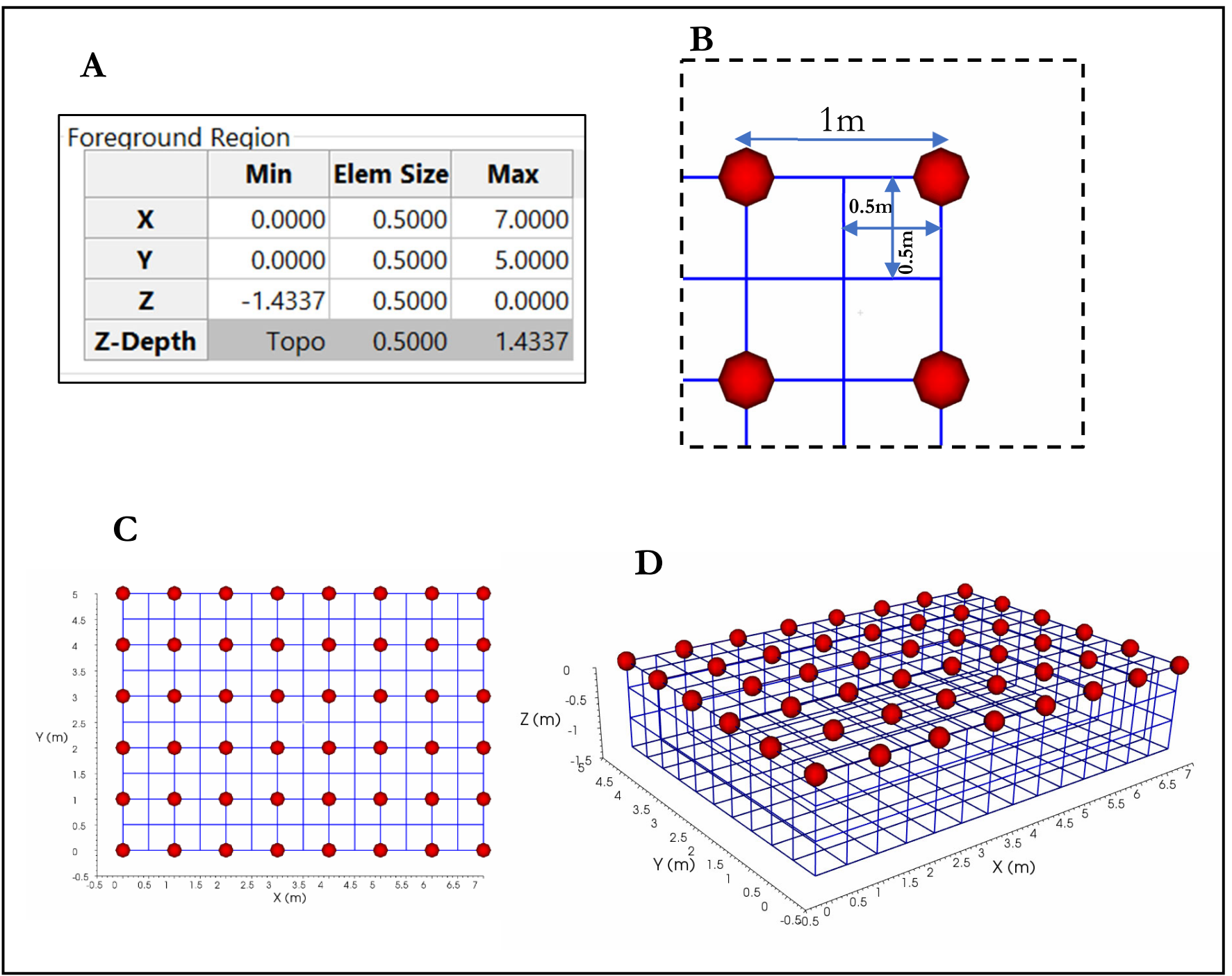
Figure 305 In A Foreground Region table. In B detail of the mesh with the size of the cell. In C e D the Foreground Region of the mesh in two different points of view

If the current settings of the Foreground Bounds does not include all the electrodes a warning is shown, and pressing the button “Correct” it is possible to be helped with an automatic adjustment.

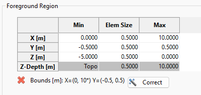
Figure 306 Foreground Bounds Warning

If the mesh can be rotated to optimize the total number of cells a message will be shown, and pressing the button “Correct” it is possible to accept the suggestion. Then, because after the Mesh Generation the rotation performed does not need anymore, it is suggested to restore the previous coordinates rotating back the dataset.

Figure 307 Rotation suggestion

In the upper part of Figure 308 an example of a mesh generated without any optimization on the rotation. It can be seen in the lower part of the image that after an appropriate rotation the electrodes will lay on the X axis so the mesh will better fit them, it will follow as final result that the Mesh size will be smaller than before.

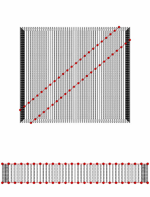
Figure 308 Example of rotation optimization

Background Region

The Background Region is the portion of the mesh which is outside the Foreground Region and defines an area necessary for the mitigation of the boundary’s effects, theoretically infinite.

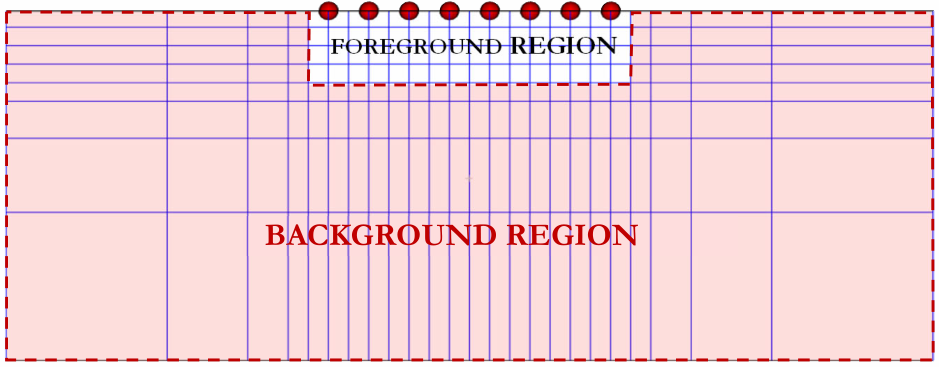
Figure 309 In red, the background region

The dimensions of the Background Region are defined by the pads: each number manage the position of a background node. The number n means n times the size of the foreground element size, e.g. if the size of the cell in X is 0.5 m, 1 mean 0.5m (1x0.5), 2 mean 1m (2x0.5), 4 mean 2m (4x0.5) and 8 mean 4m (8x0.5) (Figure 310).

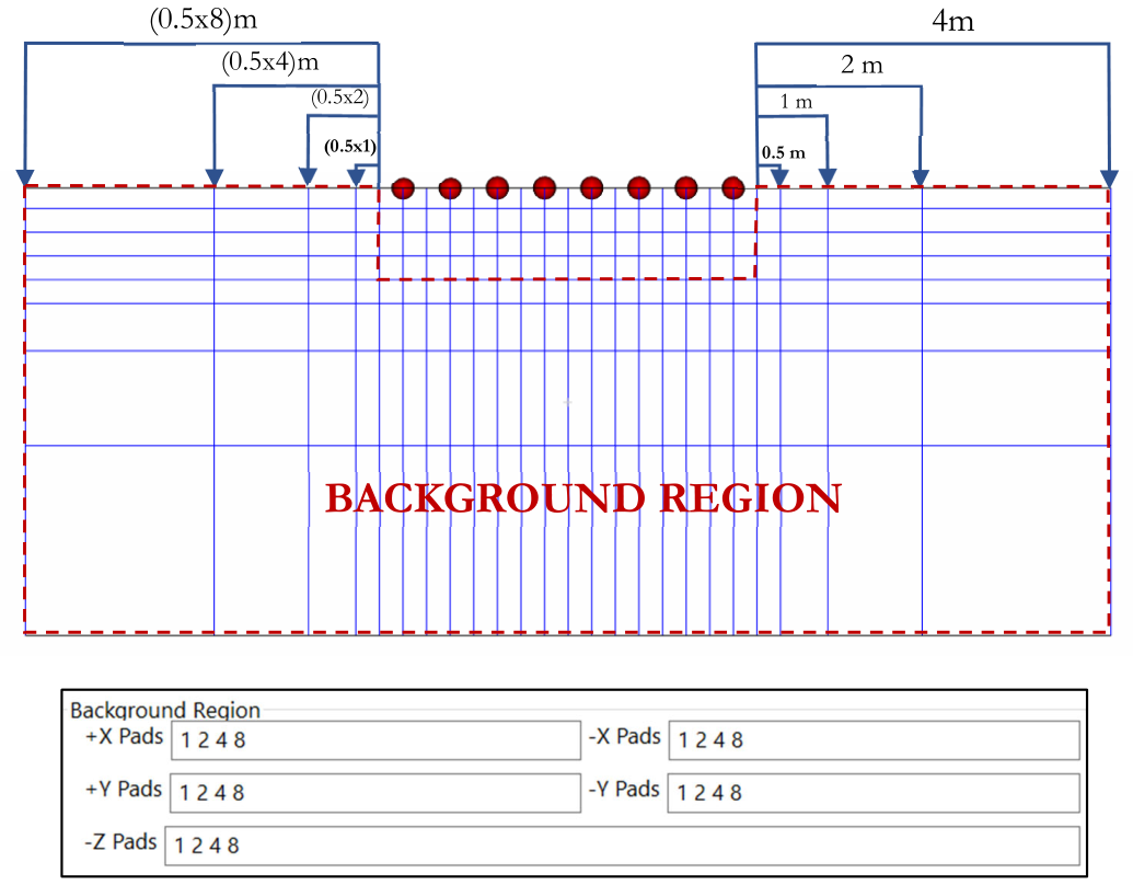
Figure 310 Definition of background limits through pads

It is possible to increase or decrease the dimensions of the background by adding or deleting the number of pads in the table. The pad numbers may be different in X, Y and Z direction. Clicking on the Compute Optimal Value button will automatically calculate the pads until 64.

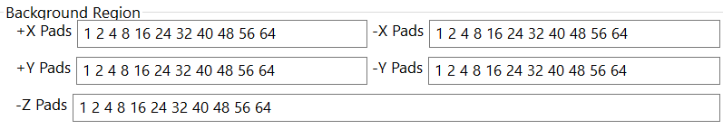
Figure 311 Pad setting

If the user changes the pads in the Background region from the automatically calculated pads he needs to make sure that the remote pole (if it exists) is included in the mesh. To do that, after generating the mesh make the remote pole visible (see section Show remote pole) and verify that it is inside the mesh. (unchecking Foreground Only tool as explained in section Plot Only Foreground).

If the current settings of the Background Bounds does not include all the electrodes (included the remote poles) a warning is shown, and pressing the button “Correct” it is possible to be helped with an automatic adjustment.

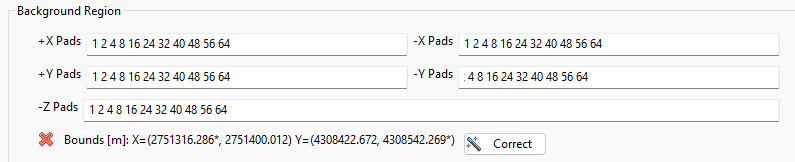
Figure 312 Background Bounds Warning

Note that the Background pads depends on the cell size, so if it is modified then it is also probably needed to check again the Background Bounds.

Model

Background value

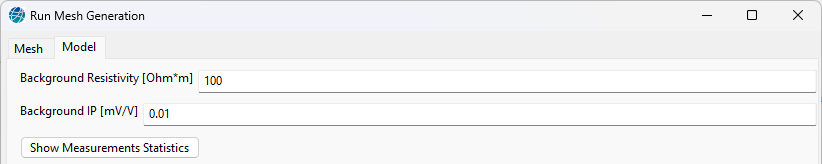
Figure 313 Background value

In the Model tab it is possible to set the Background Resistivity and IP values that will be used as starting values during the inversion process. The default values are automatically calculated through “Compute Optimal Value” function. The user can change them typing the desired values in the appropriate edit boxes. To make the right choice it is useful to consider the median and the average value in the Resistivity/IP Histogram panel (more details in section Histogram).

A quicker way to get the statistics of the measurements is to press the button “Show Measurements Statistics”.

Anomalies

Moreover, through the table, it is possible to insert one or more anomalies in the Mesh, or a known stratigraphy. Right click on the table and chose “Append Anomaly”.

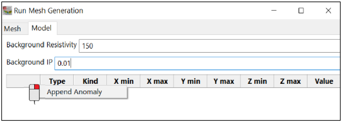
Figure 314 Append Anomaly in model table

An empty row will be added to the table to be filled with the desired values. Repeat this operation to add more anomalies. In the following example three Resistivity anomalies are added to the model. It is possible to choose the position and dimension of the anomaly setting the X, Y and Z coordinates. In the following example, the Background Resistivity is 173 Ohm*m and the Resistivity of the anomalies are 20, 500 and 300 Ohm*m.

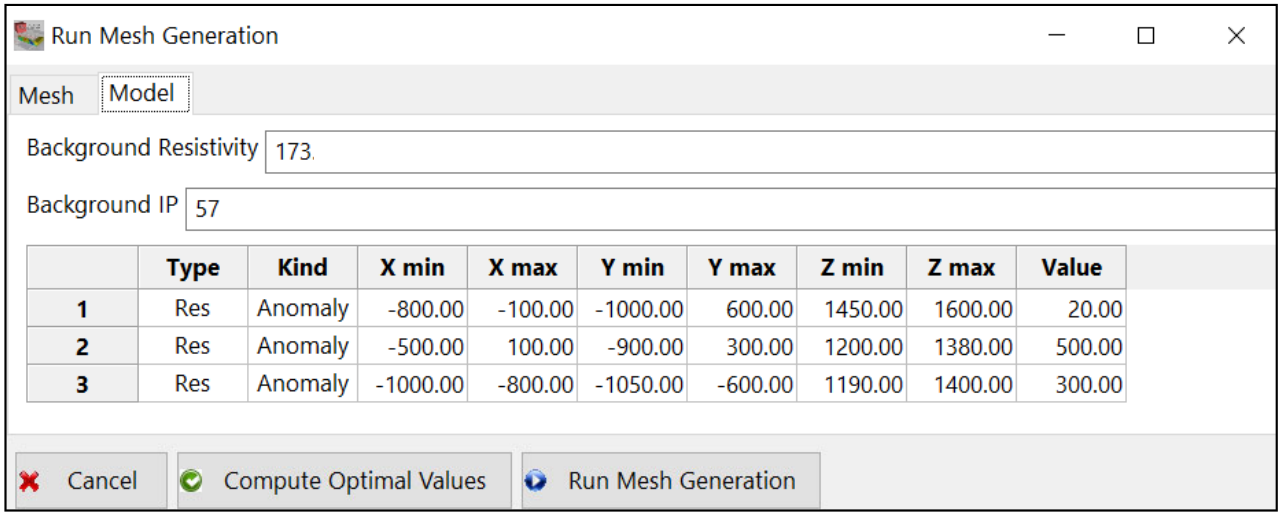
Figure 315 Three customized anomalies added to the Model

The same procedure is applicable for the insertion of IP anomalies, clicking with the right mouse button on the Type box and choosing IP instead of Resistivity.

To remove an anomaly (of any type) right click on the specific raw of the table and choose “Delete Anomaly”.

To actually take the anomalies into account during the inversion, check the “constrain to reference model” button in the inversion panel (see section Inversion Tab).

Clicking on “Run Mesh Generation” will create the mesh, once the Mesh and the Model tabs have been filled with the appropriate parameters. This process can take some processing time depending on the mesh size and the number of cells.

To customize the Mesh visualization mode use the dedicated node in section Mesh and Model. The variations of Resistivity values of the model can be displayed in several ways. Through contour lines, volumes, surfaces or sections (all these options are explained in detail in section Mesh and Model) (Figure 316).

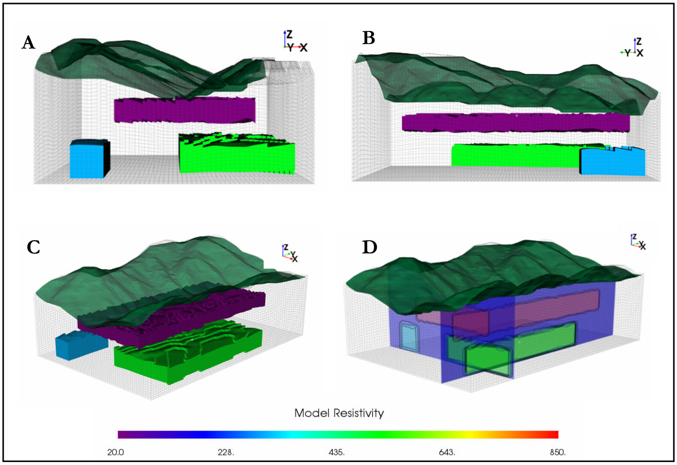
Figure 316 Example of different way to display the starting model

In the A, B, and C cases the topography (in dark green), the mesh (grey cells) and the three model anomalies (in purple, light green and light blue) are displayed as volumes, from two different points of view. In the case D the topography (in dark green), the mesh (grey cells) and the three anomalies are displayed through two vertical sections.